|
Long slender filaments or fibers suspended in fluids are fundamental to understanding many flows arising in physics, biology and engineering. Examples include fiber-reinforced composites, the dynamics and rheology of biological polymers and the motility of microscopic organisms. Such filaments often have aspect ratios of length to radius
ranging from a few hundred to several thousand. Full
discretizations of such thin objects in a 3D domain is very costly.
By applying a non-local slender body theory, an integral equation
along the filament centerline, relating the force exerted on the
body to the filament velocity, is obtained. The equation is
asymptotically accurate to An equation for the field velocity in any point away from the
filament is also obtained, to the same accuracy in The filaments we are considering are inextensible and elastic. Replacing the force in the integral equation by an explicit expression based on the shape of the filament, using Euler-Bernoulli elasticity, yields a time-dependent integral equation for the motion of the filament centerline. This equation will include the filament tension, for which an equation can be derived by using the condition of inextensibility of the filament. The evolution of the system therefore, in each time step, requires the solution of an auxiliary integro-differential equation for the filament tension. The resulting time-dependent equation suffers from an instability at small, unphysical length scales. The numerical method is therefore based on a modified integral equation that removes this instability. In our numerical algorithm, the filament centerlines are parameterized by arclength, and discretized uniformly. All derivatives are computed using second-order divided differences. Special quadrature rules have been developed to compute the necessary integrals. A second-order time-stepping scheme is used, with implicit treatment of high derivatives. A product integration method is applied to evaluate the integrals in the integral operators. We place our filaments in a shear flow. In the
non-dimensionalized equations, there are two physical parameters.
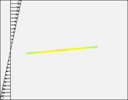
One is If one single straight filament is inserted in a plane shear
flow at some angle to the x-axis, it will simply rotate around its
center of mass. If we introduce a small perturbation to the
filament, so that it is not exactly straight, there are two
possible scenarios. Either, this perturbation will disappear with
time, and the filament will stay straight. However, if the filament
is under compression for some time, and if the value of We present short animations that show the fundamentals for this
buckling, for
Next animation is one of 15 interacting filaments, inserted into
a oscillating background shear flow,
The parameters are
Interesting phenomena to study for suspensions are filament
orientation, suspension viscosity as a function of volume fraction
and flexibility of the fibers, and normal stress differences.
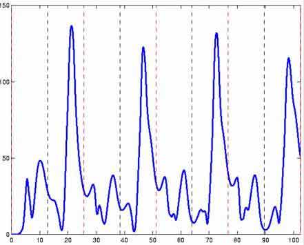
Already for one single filament in the plane, we find that as it
buckles, integrated over a full rotation, it yields a positive
first normal stress, which is not the case if buckling does not
occur. The anti-symmetric configuration |
 , where the slenderness parameter
  is the ratio between the
radius and the length of the filament.
is the ratio between the
radius and the length of the filament. , which relates the
characteristic fluid drag to the filament elasticity.
, which relates the
characteristic fluid drag to the filament elasticity. , for
three different values of
, for
three different values of  and
and  .
In these animations, the filament has been colored with the line
tension. The line tension changes from negative to positive, as the
filament goes from being under compression to being under
extension. We can note that if the initial configuration x
is reflected to -x, it will evolve under the symmetry
.
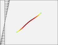
In these animations, the filament has been colored with the line
tension. The line tension changes from negative to positive, as the
filament goes from being under compression to being under
extension. We can note that if the initial configuration x
is reflected to -x, it will evolve under the symmetry  . Hence, if we change the
sign of the perturbation, the filament will buckle in the other
direction.
. Hence, if we change the
sign of the perturbation, the filament will buckle in the other
direction.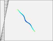
 . We impose periodic boundary conditions in the
streamwise (x) direction. The animation shows one period in
time.
. We impose periodic boundary conditions in the
streamwise (x) direction. The animation shows one period in
time.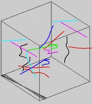
 and
and  . We use
N=100 points to discretize each filament, and a time step
. We use
N=100 points to discretize each filament, and a time step  =0.0128.