Model
Practicals -
Stochastic Climate Models
- Students should first
review the lecture notes for this subject which can be downloaded here.
- The programs for this model all reside on the server
woodend.cims.nyu.edu
and students have a user id students. In
order to login you need (for security reasons) to be within the CIMS
network and you need to login using ssh. To
do this issue ssh students@woodend.cims.nyu.edu
from a cims machine. When prompted enter the password issued in class.
Do not share this password.
- The stochastic model codes may be found in
/home/students/models/stochastic
and students are asked to copy this sub-directory and its contents to
their own subdirectory to avoid clashing with other students in the
running of the model.
- To invoke the model gui type
matlab -nodesktop
and then type stochint at the matlab prompt.
The following display should appear:
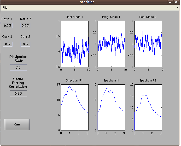
- The
model parameters should be cleared by resetting values.
- The
top panels are the time series for the real and imaginary components of
the first mode and the real component of a second mode.
The bottom panels shows the corresponding spectra. A spectral window is
used as a smoother of the spectrum since the time series are relatively
short.
- The first mode is assumed to have period of 1 time unit. The parameters have the following meaning. Ratio 1 : Decay time of mode 1. Ratio 2: ratio of the period of mode 2 to its decay time (second decay time =r2*t2). Dissipation ratio: Muliply
the decay time of mode 1 by this to get the decay time of mode 2.
Notice that the period of mode 2 is defined implicitly by these
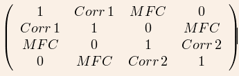
parameters. Corr 1: The correlation of stochastic forcing onto the real and imaginary and real parts of mode 1. Corr 2: Same as Corr 1 but for the second mode. Modal Forcing Correlation (MFC): A correlation parameter between the two normal modes. The four by four covariance matrix has the form
- Students need to complete the assignment which was handed
out in class. It can be download here.