Model Practicals
On the course website, students can download the quasi-geostrophic ocean-basin model (written in Matlab and stored as a zip file). All the Matlab files are prefixed by qg_, meaning quasi-geostrophic. To configure any particular experiment, as required in the exercises, the user needs to first edit the file qg_parameters.m . To run the code, the user gives the command qg_driver in the Matlab command window.
The model describes barotropic flow in a beta plane
basin forced by a prescribed Ekman pumping distribution. The model
integrates the barotropic quasi-geostrophic potential vorticity
equation normalized as in Eqn. (2.3.2) in Pedlosky (Ocean Circulation Theory):
d(D^2(psi))/dt + di^2 J(psi,D^2(psi)) + dpsi/dx =
                we - ds D^2(psi) + dm^3 D^4(psi)
where: psi = streamfunction;
we = Ekman-pumping distribtion;
J = Jacobian operator in (x,y);
D = del operator;
L = basin width;
di = delta_I/L;
ds = delta_S/L;
dm = delta_M/L.
The underlying PDEs have been non-dimensionalized,
as has been the forcing. The model domain is, generically, [0..1]
west-east (along the x-axis), and [0..1] south-north (along the y-axis). The equations are depth-integrated.
The numerical method is simple, second-order
centered finite differences with 2nd-order Runge-Kutta integration in
time. The model integrates in non-dimensional time to 100, which is
generally adequate for a spin-up from rest and achievement of steady
state.
Using the default settings, and running the model, produces four Matlab figure panels:
- Panel
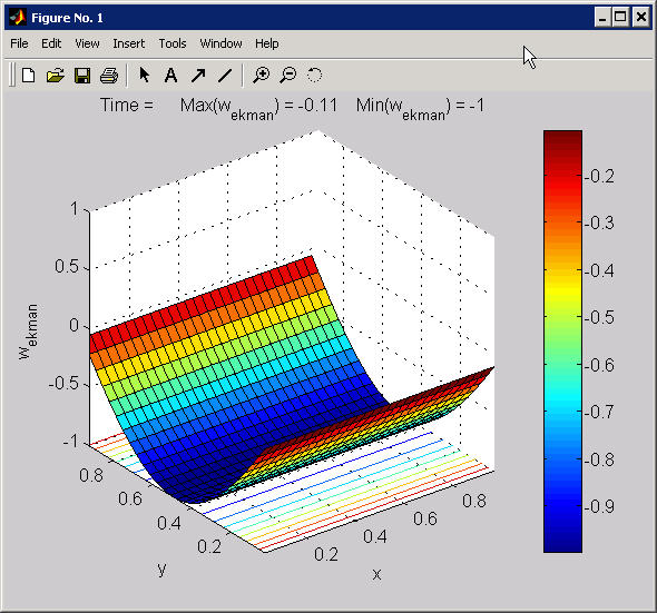
Figure No. 1: Shows a
perspective view, from the southwest, of the imposed Ekman pumping
velocity. The non-dimensional amplitude is approximately 0.1. This
forcing field is time-independent.

- Panel
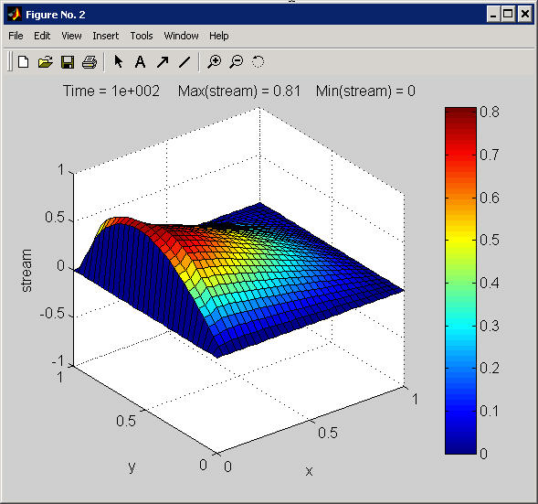
Figure No. 2:
A perspective view of the modeled stream function. As the model
integrates forward-in-time, this panel is updated whenever the
non-dimensional time is a multiple of 10. The figure shown here is the
streamfunction result at the model end (non-dimensional time is 100).
The streamfunction is intensified in the western boundary region (i.e.,
near x=0).

- Panel
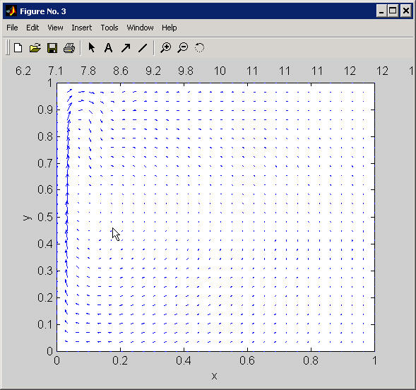
Figure No. 3:
A plan view of the modeled flow (shown as vectors). The vector field is derived by taking the perpendicular gradient of the streamfunction (from Figure 2).

- Panel
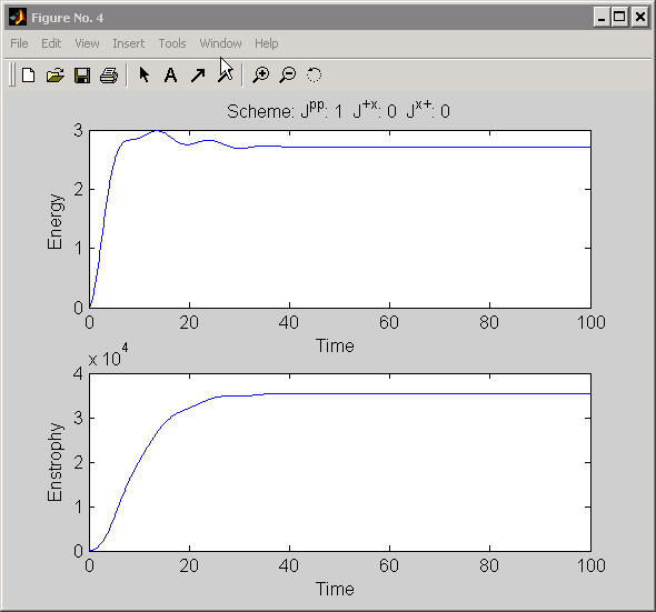
Figure No. 4:
Time series showing the evolution of the modeled kinetic energy and
enstrophy. The title of the figure refers to the particular form of the
Arakawa-Jacobian used for calculating the non-linear advection terms.
See the model code for details.

The user modifies the default parameter settings by editing the file qg_parameters.m.
The principal parameters to edit are those relating to the
non-dimensionalized size of the Stommel, Munk, and Inertial scales. The
default is to have a non-zero Stommel (bottom-friction) scale, and zero
Munk (Lateral friction) and Inertial (non-linear advection) scales.
These non-dimensional scales should always be less than 1, and are
generally of size 0.01.
The Beta-effect is activated by setting the parameter beta_effect = 1. Setting this to zero gives an f-plane model.
The Ekman pumping is activated by setting the parameter ekman_pumping = 1.
Setting this to zero gives an unforced model. This can be useful, for
example, for the case of starting the model with a non-zero flow field
and observing the decay of the flow.
The model is run with either slip or no-slip
boundary conditions, independently specified on each boundary segment,
e.g., setting slip_w = 0 for the western boudnary to be
no-slip. These lateral boundary conditions are set by the user in the
parameters file. They only have meaning in the context of a non-zero,
Munk-scale experiment.
The numerical Jacobian is formulated in a variety of
manners. The default is a non-energy conserving, but rather simple
form, as:
J(psi, zeta) = (u zeta)_x + (v zeta)_y.
The user edits the parameters file to change the type of Jacobian.
Last Modified Aug/30/2004.
©
David Holland.
All Rights Reserved.
|

|
If you would like further information
concerning any of the above topics
please send email
.
|
